MAKING SENSE OF 2D DATA – PART 2: FOLDS
This post is the second of three parts (for parts 1 and 3, see here and here) and describes the different appearances which folds can have depending on the orientation of the surface on which they are exposed.
Visualising complex objects in three dimensions isn’t easy, although geologists are better at this than most. Two dimensional objects are an order of magnitude easier to comprehend. Where the object under study is complex we can gain an understanding by visualising or portraying two dimensional slices across it. This works well because in the real world the view that geologists usually get of rock structures is on planar or approximately planar surfaces: the surface of the earth, the joint or bedding controlled surfaces or a rock outcrop or the arrays of close-spaced holes drilled along a section across an ore body.
There are potential traps in interpreting 3D shapes and relationships from 2D slices across it. I will illustrate some of these problems with specific examples involving faults and folds in rock surfaces that a mining geologist will see in surface outcrop, open cuts and diamond drill core.
This post is in three parts. Part one deals with faults and sense of movement indicators. In this part I describe problems interpreting folds using an example of correlating geological interpretation of surface maps and drill sections. Part 3 is also concerns folds but specifically the interpretation of small folds exposed on the cylindrical surface of diamond drill core.
I have no doubt that many experienced geologists will find my examples and explanations self-evident, trivial. But bear with me, not all geologists are experienced, not all spend much time interpreting maps and drill holes, and even non-geologists might find the examples instructive.
Below is a map of a 150 meter deep open cut gold mine in Western Australia. The deposit was first mined as a high-grade underground mine in the 1890’s and again in the 1930s. It was re-activated as an open cut mine in the 1990s.
The geology exposed on the walls and floor of the pit is projected onto the horizontal map plane. This is a very common and useful way of representing outcrop in an open cut. It is a composite view of all exposures whether seen on horizontal surfaces such as benches and pit floor, as well as on steep-dipping surfaces such as batters. The resulting map is a useful tool that can be taken into the pit to explain the nature of everything seen, but, as the example shows, it needs to be interpreted with care. The only alternative to such a map would be a stacked series of Level Plans or a series of vertical strip plans of exposures on the steep batters.
Note that on the map below the outlines have been smoothed to remove the “stepping” effect of the pit wall benches. North is to the right.
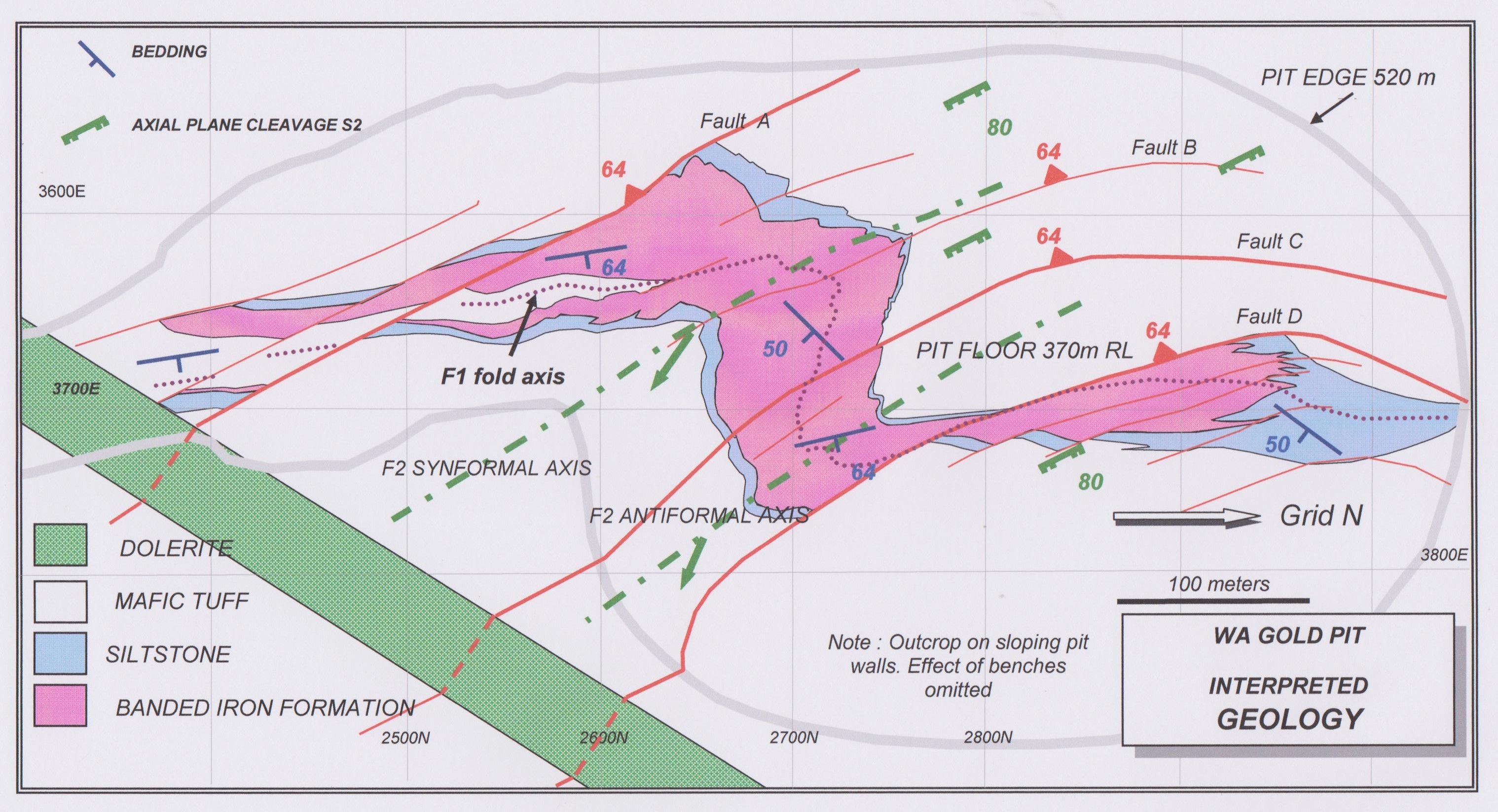
Host rocks are a sequence of mafic volcanics. A thick, S-dipping, banded iron formation (a metamorphosed iron-rich sediment consisting of interbedded jaspilite and magnetite, usually referred to as BIF) forms a prominent marker bed. The rocks are affected in the pit by a prominent Z-profile fold pair with steep, SE-plunging axes. All rocks, apart from the dolerite, are cut by a series of steep SW-dipping reverse faults, the most prominent of which (Fault D) cuts the BIF with wide zones of pervasive sulphidation, silicification and gold mineralisation (a picture of the high-grade gold ore from this deposit can be found on my Home page). Many instructive mineralisation stories can be made from this deposit: how sulphidation has selectively replaced magnetite horizons (thus raising ph of fault fluids and triggering gold deposition), how Fault D is a tight, unmineralised, ductile structure where it cuts mafic rocks but broadens to a wide brittle fracture zone in the competent BIF: but I do not want to enlarge on these stories here. Instead, I want to draw your attention to how different the shape of the fold looks in the vertical E-W drill Section below compared to the map view above. 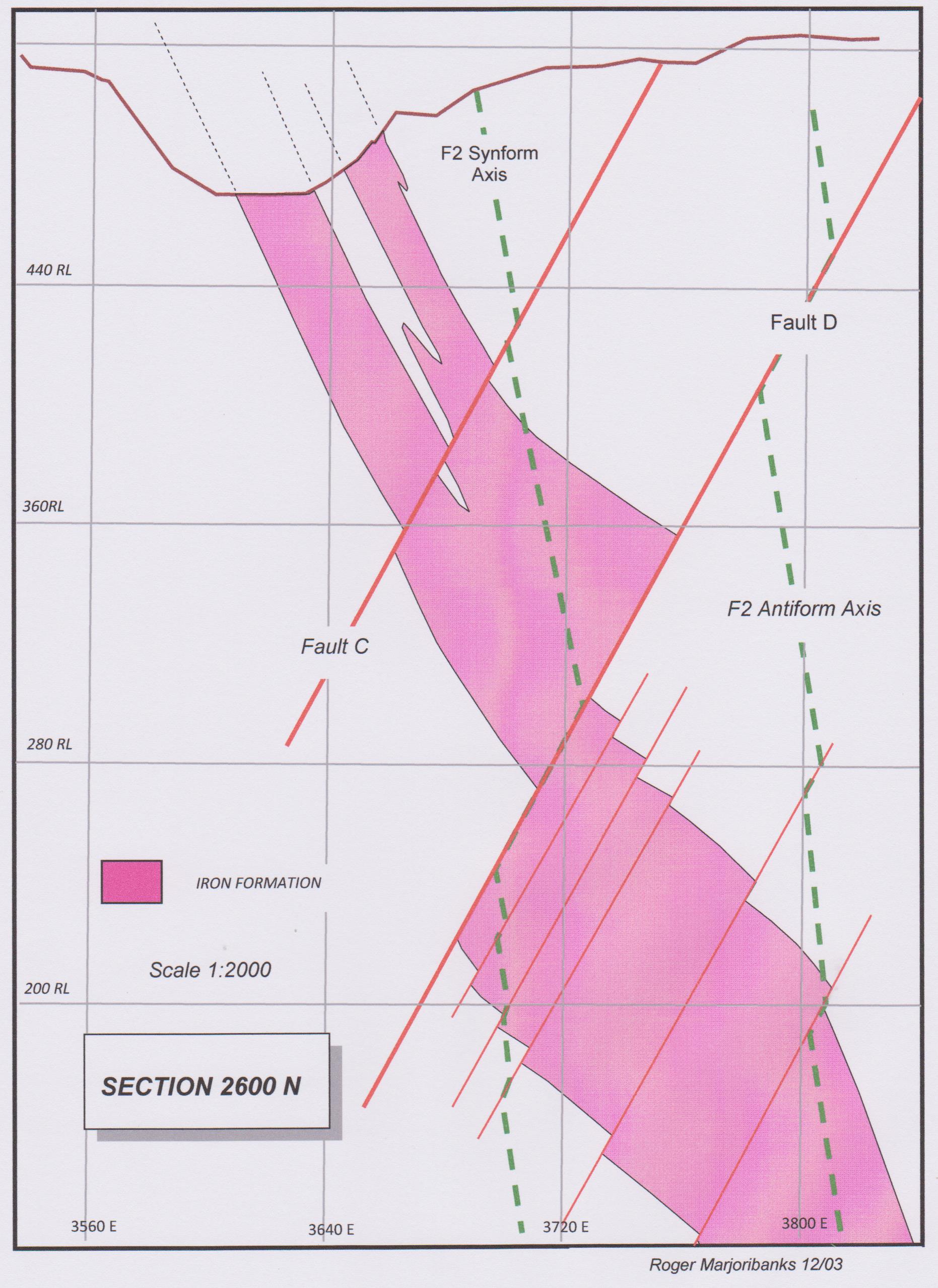
What has happened to the tight F2 fold that was so prominent on plan view? Why do the folds appear to have an interlimb angle of 90° on the plan but around 160° on the section?
There are two reasons, each contributing about equally to this effect:
- The map shows outcrop across a hole with steep sloping sides. The north trending limbs of the fold are essentially parallel to the walls or the floor of the pit: the trend of the outcrop on these limbs is thus more or less parallel to strike. The short common limb of the fold however outcrops down the steep west wall of the pit so the outcrop trend of this limb is not parallel to strike, but is a composite trend between strike and dip directions. This gives the short limb a more easterly trend and makes the fold on the map appear tighter than it really is. If you look at the symbols for actual measured strikes on the map it is apparent that the true interlimb angle (i.e. the angle between the two limbs measured on a plane at right angles to the fold axis) is around 120°.
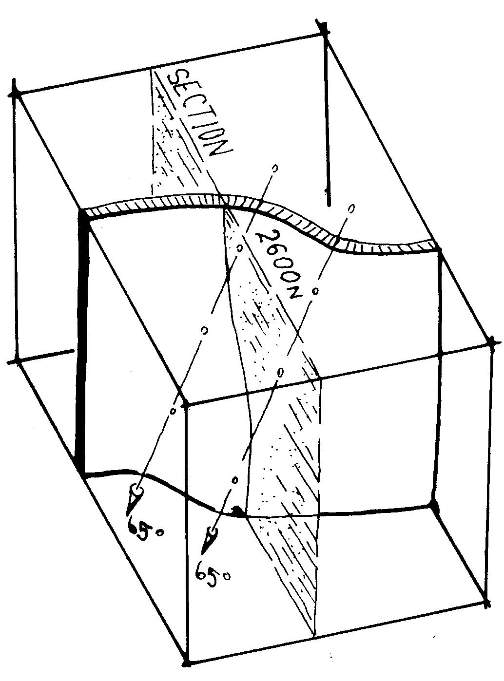
- The folds plunge 65° to the SE. In other words, the map represents is a slice at 65° to the fold axis: the vertical section however cuts the fold axes at 25° . The map thus is much closer to a true fold profile than the section. The difference on the fold shape shown by the two differently-oriented planes can be understood by reference to the block diagram below:
The take-home message is this: 2-D slices through complex geological objects can only be interpreted if some information about the third dimension is also provided.
Note: this blog no longer accepts comments as an on-line forum (there was too much Spam coming in!). However, if you want to contact me about any blog post or subject with opinions, criticisms or comments please use the email forms provided in the Contact tab of the site.