Making sense of 2-D Data – Part 1: Faults

Visualizing complex objects in three dimensions isn’t easy, although geologists are better at this than most. Two dimensional objects are an order of magnitude easier to comprehend. Where the object under study is complex we can gain an understanding by viewing it on two dimensional slices or sections across it.  For geological objects the sections most commonly employed are horizontal (otherwise known as maps or plans) and vertical. Complex problems of correlating and interpreting structure can then be solved in 2D space. By stacking a series of parallel sections or maps through the geological object, a full 3D picture can be built up[1].  This works well because in the real world the view that geologists usually get of rock structures is on planar or approximately planar surfaces: the surface of the earth, the joint- or bedding-controlled surfaces or a rock outcrop or the arrays of close-spaced holes drilled along a section across an ore body.

There are potential traps in interpreting 3D shapes and relationships from 2D slices across it. I will illustrate some of these problems with specific examples involving faults and folds in rock surfaces that a mining geologist will see in surface outcrop, open cuts and diamond drill core.

To avoid making the post too long I will divide it into three parts.  Part one deals with faults and sense of movement indicators. Part 2 covers folds using an example of correlating geological interpretation of surface maps and drill sections. Part 3 is also about folds: but specifically about small folds seen on the surface of diamond drill core.

 I have no doubt that many experienced geologists will find my examples and explanations self-evident, perhaps trivial.  But bear with me, not all geologists are experienced, not all spend much time interpreting maps and drill holes, and even non-geologists might find the examples instructive.

The interpretation of faults usually involves working with maps and sections.  Judgements  have to be made on sense-of-movement by the displacement which the fault makes on tabular lithological markers such as sedimentary beds, veins or dykes.  The shear direction, or relative displacement across a fault is known as the Fault Movement Vector (which we will here call M). M is a vector so it has a direction as well as an attitude.  It is shown graphically on a map or a section by an arrow. Two parallel but opposed arrows are used to show the movement, relative to each other, of the rocks on either side of the fault. You can find a much more detailed discussion of fault movement vectors in my post “The movement of faults” (Structural Geology Category).

The line of intersection of a marker bed with a fault plane will be referred here to as I. The most important point to take from this discussion is that the amount of displacement of a marker bed across the fault is a function of the angle which the Fault Movement Vector (M) makes with I. If the angle is high then the displacement of the Marker Bed will be high with maximum displacement occurring when the angle is 90°.  If the angle is 0° (i.e. where M is parallel to I) there will be no apparent displacement of a tabular bed across the fault. 

Finally, if all we have is 2D information, the above is all we can know about the displacement across the fault.

I will illustrate this with two examples, starting with the geological map below:

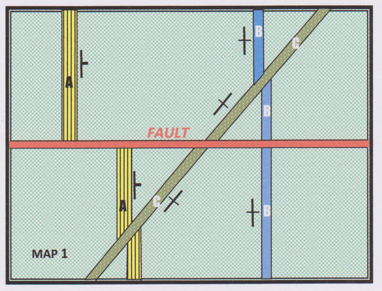
On the map are three tabular, north-striking, marker lithologies labelled A, B & C.  They are cut by an east-west fault of unknown dip. The only 3D information available (deduced from the way the outcrops trend across an incised landscape) is that unit A dips to the east and units B and C are vertical. With this information, what can we say about the movement on the fault?  Quite a lot, even with this limited information because (1) we have some 3D information and, (2) the fault affects several variably-oriented marker units.

Consider Unit B: The vertical unit shows no displacement across the fault. Does this mean that there is no displacement? No –only that a homogenous bed with uniform thickness and this particular geometry is incapable of showing the displacement. We can deduce that geometry: the fault movement direction (M) must lie at 0° to I – the trace of B on the fault plane. That is, M lies along the dip of the fault. This establishes that fault movement was dip-slip, but not which is the up-thrown side of the fault, and which the down-thrown side.  The amount of this movement is undetermined.

Consider Unit  A:  The east-dipping  unit A shows a left-lateral (or sinistral) displacement across the fault, suggesting strike-slip movement. However, we know from Unit B that the true movement on the fault was dip-slip, so the map displacement of A is misleading.  A north-block-down dip-slip movement on the fault will cause just such an apparent sinistral displacement on a plan view.  If the fault dips to the south, it is a reverse fault: if to the north, a normal fault. Not knowing the exact dip of A means that the amount of movement is undetermined.

Consider Unit C: This is clearly an intrusive rock, possibly a dolerite dyke. Unit B is displaced across it but note that the truncated ends of B can be matched orthogonally (i.e. at right angles to the dyke margins) across the dyke. This indicates that the dyke has intruded by occupying an extensional zone (a pure shear extensional fault) that opened in a direction at right angles to its margins. This is a characteristic mechanism of dyke intrusion.

The apparent strike-slip displacement of unit B across unit C is misleading.

Bed C shows a small, apparent, right-lateral (dextral) displacement across the fault.  Yet we know from Bed B that fault movement was pure dip-slip. How do we explain the displacement? There are two possibilities.

1. The dyke is not actually vertical but has a high angle dip to the west (i.e. the opposite sense from Bed A). North-block down fault movement (which we determined from its effect on A & B) will therefore cause a slight apparent dextral displacement of C.  In the real world this would be a valid, even compelling, interpretation, but this is an exercise and we are given that the bed is vertical, so there must be another explanation… 
2. During fault movement, rocks to the north of the fault have moved closer to the rocks on the south.  This can only happen if there has been a loss of material in the fault zone. This is a typical effect of faults and is caused by pressure solution during fault movement: rock material is dissolved from the face of the fault is carried away by hot fluids to be deposited elsewhere in the fault as veins of quartz or calcite in zones of relative tension.  This leaves behind an insoluble clay residuum known as fault gouge.  The effect of moving together the two truncated ends of a unit is to cause an apparent strike-slip offset (so long as the unit is cut by the fault at any angle less than 90° to the fault trace.  We deduce that a small component of compressive pure shear movement operated at a high angle to the fault plane.

Now for my second geology map example:

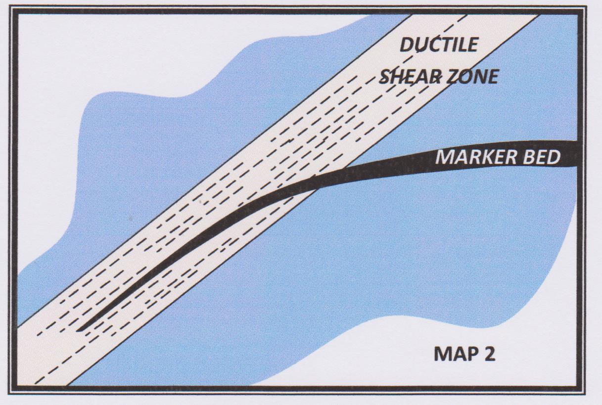
Note, there is no scale on this map. The horizontal surface shown could represent an area of many square kilometres. It could also be a sketch of a typical sense-of-movement indicator – a few centimetres across. The sort of evidence that you might use in the field to attempt to determine the movement on a fault[2].

MAP 2 shows a marker bed strongly deflected and progressively thinned into a ductile shear zone. What can we say about the movement direction on the shear zone? Only this: because of the strong deflection, the angle between the trace of the marker bed on the shear zone (I) and the movement direction M must be large. Since neither M nor I is known we can say nothing more without some 3D information. It may seem at first glance that there is at least a component  of left-lateral strike-slip fault movement, but this would only be the case if I is steep plunging.  If I has a shallow plunge, then M must be steep plunging. In this case the situation shown in the block diagram below might apply.

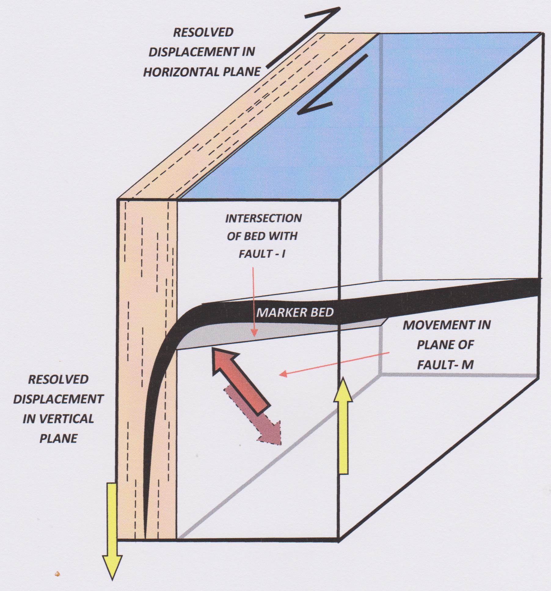
When full 3D information is available we see that I has a shallow plunge and the Fault Movement Vector (M) is steep-plunging with an oblique-slip movement (large red arrows) . This can be resolved into a 65% east-block-up dip-slip component (shown by opposed yellow arrows on the vertical face of the block diagram) and 25% resolved right-lateral strike-slip movement (shown by black arrows on the top, horizontal face). The apparent left-lateral drag on the marker bed on horizontal view is caused by the dominance of the vertical shear component acting on a shallow-dipping marker. This is the same misleading apparent displacement that we saw displayed by Unit A on our first example of Map 1. 

The take-home point is that to correctly interpret fault displacement vectors, whether using displaced marker beds at map scale or outcrop-scale sense-of-movement indicators, you need at least some 3-D information.

 

Note that this blog does not accept comments any more (there was too much spam coming in). However, if you want to contact me you can email me direct using the address under the CONTACTS Tab.