Sense of movement structures – Part 1, Theory

Sense of movement structures in fault zones - Part 1, Theory

Within or adjacent to fault zones, various minor associated structures can be present that enable the sense of movement across the fault to be determined. These structures are called movement or kinematic indicators.

Faults are the host to epigenetic, vein-type metal deposits. Identifying the nature of a fault and the sense of movement across it enables prediction of the likely shape and attitude of any high grade ore shoots that might be associated with it (see my previous post on drill hole targeting). One of the best ways to determine sense of movement (also called the movement vector or the kinematic indicator) is through associated indicator structures that can be observed in outcrop and drill core. Some large movement indicator structures or patterns of structures can also be identified at map scale.  This post describes these structures: why they form, what they look like and how they can be interpreted.

This post is in three parts. Part 1 gives the theory of  how sense of movement structures form and their kinematic significance. Part 2 provides illustrations of actual structures from exposures in the field, in mines and in drill core, while Part 3 provides a tabulated summary of the objective criteria by which the different classes of sense-of-movement structure can be identified and interpreted.

Stress and Strain

Structures in rock are an example of deformation.  Another word for deformation is strain. The strain that you observe is the cumulative effect of forces that acted on the rock over time.

A force acting on any given point in a rock is known as stress. Strain is the tangible effect that you observe: stress is the intangible cause that can only be deduced. However, the relationships between strain and stress are well known and provide a high level of predictability to structural geology. Higher, at any rate, than many other areas of geological science.

Every point in a rock is acted upon from all directions by stresses. However, because the infinity of stresses will, to various degrees, tend to cancel out or reinforce each other, they can all be resolved mathematically into just three stresses that are mutually at right angles to each other. The three orthogonally arranged stress directions are known by the Greek letter sigma (written thus: σ). Ignoring the gravity vector, in most rocks, in most places and at most times the three stress axes will be of approximate equal magnitude – a state is known as isostatic stress.  However, tectonic movements, isostatic adjustment or heat flow can lead to the stresses being locally unequal.  When this happens it is called deviatoric stress. Deviatoric stress causes rock structures to form.  With deviatoric stress, the direction of greatest stress is called σ1 (sigma one); the direction of least stress is called σ3 (sigma three) and the stress with an intermediate value is called σ2 (sigma two).

 

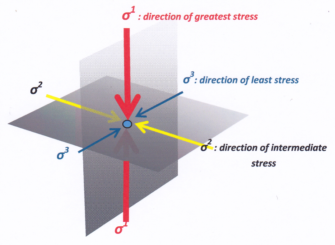
Figure 1: Graphic showing the three principal directions of resolved stress that act upon every point of a rock in the ground that is subject to deviatoric stress. Sigma 1 is always positive. Sigma 3 and sigma 2 are usually positive but may be locally negative.

For reasons that should be sufficiently obvious, the bulk of rock deformation takes place as a result of the stress difference between σ1 and σ3. This means that, for most practical purposes, we need only show deformation in the plane containing these two axes. This is called a “plane strain” analysis. It is a simplification, but a useful one. It means that we can illustrate stress-strain relationships with two-dimensional diagrams in the plane of sigma 1 and sigma 3, as in the graphic below.  On the diagram the stress axes sigma one and sigma three are shown as arrows, the lines represent planes – potential rock structure – that extend into the page parallel to σ2.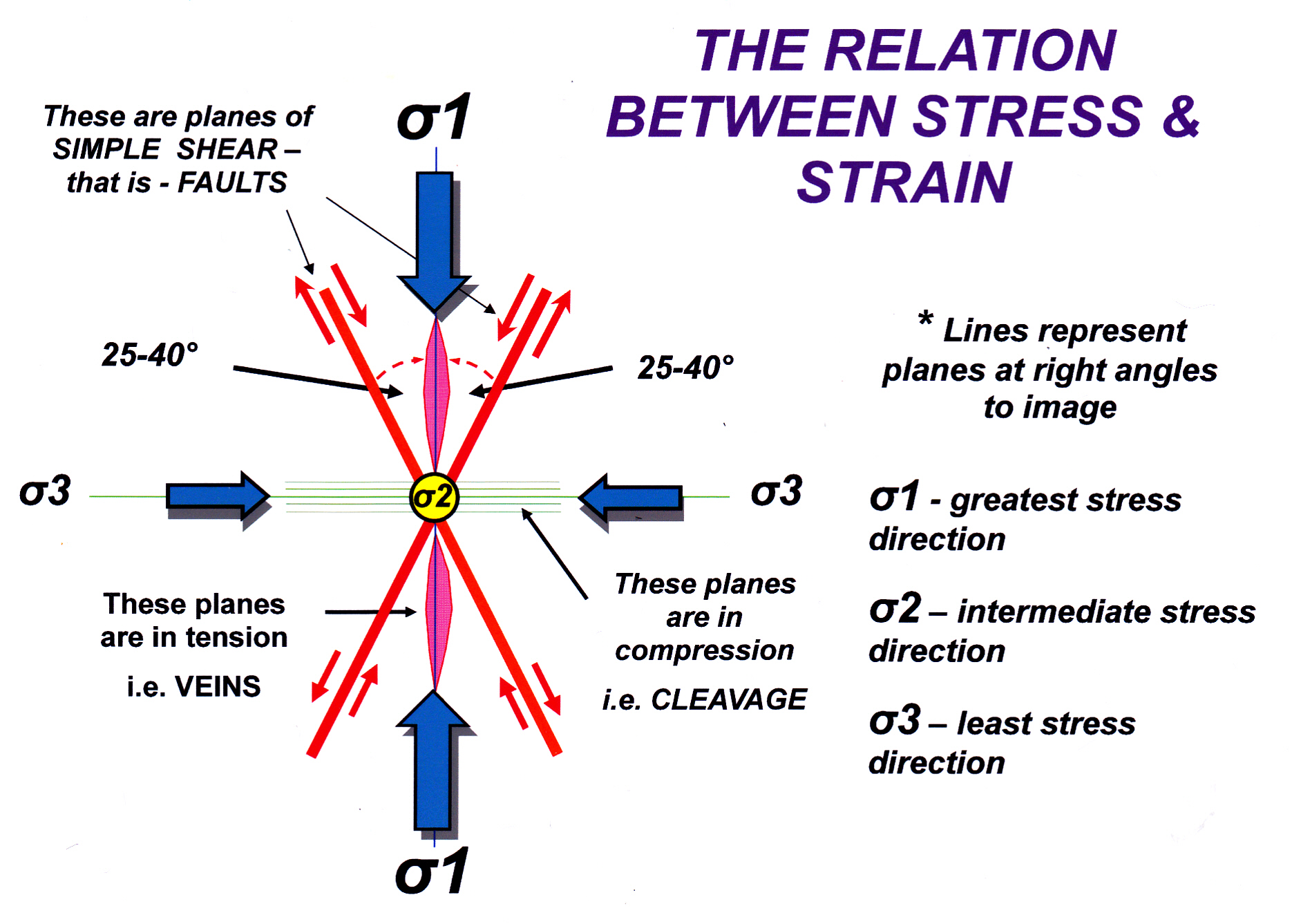

Figure 2: Structures that may form in the plane containing the principal (σ1) and least (σ3) stress axes. The intermediate stress axis (σ2) is normal to the page. Red green and purple lines show structures that might form and their angular relationships to the stress axes.

This diagram should be familiar to anyone who has gone through a university course in structural geology: yet it is widely misunderstood. I have been asked: “how can you simultaneously get compressive and extensional structures in the same rock?” and: ” how can two faults cross each other in the form of an X, and yet neither displace the other?”.  The answer is, you can’t, at least not in the same rock, at the same place and at the same time. That is not what this diagram means.  The graphic is a  representation of the mathematical formula which predicts the attitude of planes where the maximum amount of shear force will be resolved, given two primary stress axes of unequal value. Whether any structures  actually form in a stressed rock, as well as the type and mix of structures,  is dependent on other factors such as the difference in magnitude between σ1 and σ3, the strength of the affected rocks, the temperature and  the rate at which stress is applied. But given that a particular structure will form, the diagram predicts what its attitude will be relative to the stress axes.

Theory, mathematical computation, experimental laboratory rock deformation and field observations have established that:

• Planes that lie at right angles (normal) to σ3 will be planes of relative tension: in rocks such planes might be marked by open brittle fractures or joints, or (more likely) by fissures filled with vein material or igneous dykes and sills.
• Planes which lie at right angles to σ1 will be planes of relative compression: in rocks, such planes will be cleavage or stylolites or perhaps fracture zones coated with clay or graphite indicating that material has been lost by pressure solution from the sides of the fracture (the clay, or fault gouge, is an insoluble residuum of this process).
•  Planes which lie at angle of between 25°- 40° to σ1 are planes that have the maximum  resolved component of simple shear across them[1].  Simple shear is where the rock on one side of a fracture moves laterally with respect to the opposite side. The exact angle depends on the nature of the rocks being deformed with the smaller angle being a feature of shears in stronger (more competent) rock such as quartzite. The higher angle characterizes shears forming in less competent rocks such as siltstone. These planes in actual deformed rocks may become simple shear faults.

Structures in Zones of Simple Shear

Real faults are not mathematical planes: as well as length and breadth they have a width which may range through many orders of magnitude. All faults are tabular fault zones. Consider one of the red lines – a potential fault zone – on the diagram above.  The amount of relative  movement between the two sides of the zone could be a few millimeters or hundreds of kilometers. Structures which can show the sense of movement are second order structures which occur within, or immediately adjacent to, the fault zone. To understand these structures we therefore need to consider the stress and strain that exists within an actively moving fault zone.

The fault zone itself is the primary structure caused by a Primary or First Order Stress Field.  However, within the zone itself, the shear movement re-orients stress axes to a new orientation called Second Order Stress. Second Order stresses produce second order structures that reflect the movement direction.

At this point it is useful to introduce the idea of the Strain Ellipsoid. This is a mathematical concept, but one that is easily visualized in geometrical terms. Think of a sphere of perfectly elastic (squashable) material such as rubber ball. This sphere represents a rock in its undeformed (unstrained) state. Now subject the ball to a tri-axial stress field : it will compress most in a direction that is parallel to σ1: the material displaced will extend the ball in the other two dimensions most noticeably in the direction where it is least constrained, i.e. parallel to σ3. As a result, the sphere becomes an ellipsoid, called the Strain Ellipsoid. The strain ellipsoid does not represent an actual rock structure (perfectly elastic spheres do not exist in nature): it is a graphic which illustrates the mathematical relationship between stress and strain.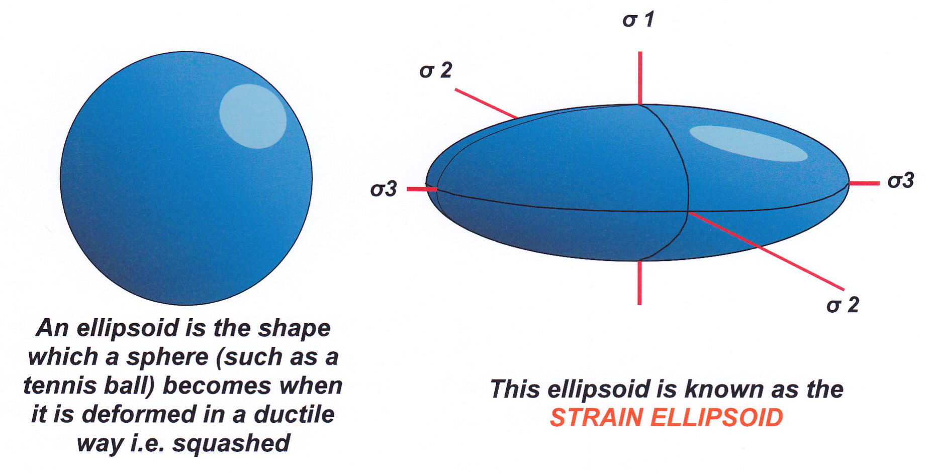 

Figure 3. The effect of stress on an imaginary unit sphere.

In simple shear zones, we only need consider the section through the ellipsoid that contains σ1 and σ3 axes. This section is the strain ellipse.

Now consider what happens inside a simple shear zone[2]. A good model for such a zone is a deck of cards on the end of which two lines and a circle have been drawn, as shown in left diagram below.

 

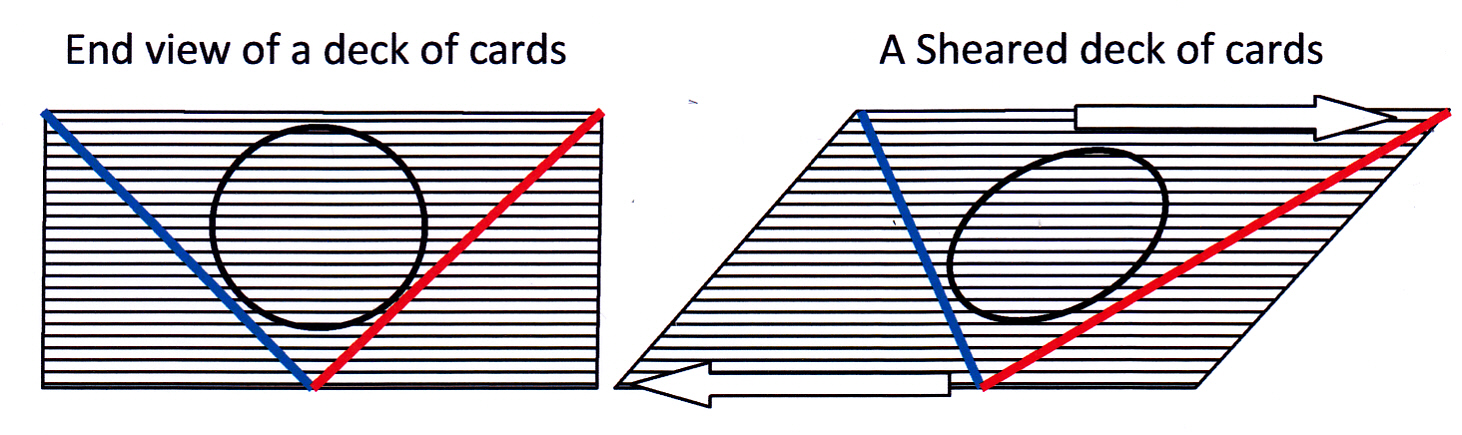
Figure 4: A deck of cards provides a useful model to illustrate the strain effects of simple shear.

Now we push the deck sideways by sliding each card to the right over the one below by the same small amount . The end face of the deck now has a trapezoid shape as shown at right, above. We have applied a dextral simple shear rotational force across the pack.  The resulting strain is entirely two dimensional (or monoclinic) as no deformation has taken place at right angles to the page. The blue line inscribed on the undeformed pack that formed an original acute angle with the direction of shear is now shortened by the shear movement.  It has thus undergone a compressive strain. The red line, whose initial orientation formed an obtuse angle with the shear direction, is extended by the shearing (extension strain). The initial circle is deformed to an ellipse whose long axis is tilted in the direction of shear – this is the strain ellipse. It easy to show mathematically that those lines that were initially at 45° to the boundaries of the shear zone will show the maximum amount of strain – either a shortening or an extension – depending on their original orientation relative to the shear direction. From this we can deduce that within a zone of simple shear (i.e. within a fault zone) the principal and least stress axes (σ1 and σ3) must, at every given moment during deformation, be oriented at 45° to the boundaries of the zone.

At last we get to the killer diagram, one that has graced a dozen textbooks and a hundred learned papers. Here it is in simplified form:

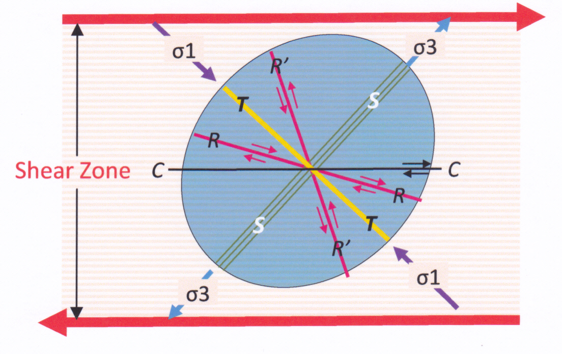
Figure 5. Graph showing orientation of greatest and least stresses (σ1 and σ3) within a zone of simple shear (i.e. a fault zone). The blue ellipse is the strain ellipse that exists at every instant during shear (known as the instantaneous strain ellipse). The orientations of the various rock structures which can form are shown. Compare these with figure 2.

S – (green lines) these are planes of compression – they could be ductile foliations of various kinds, the axial planes of folds, even stylolites. The angle which they make with the zone boundaries forms an obtuse angle with the direction of shear (i.e.  the surface is congruent with the movement direction). This gives the sense of movement.

T – (yellow) these are planes of tension. They are sometimes characterised as E (for extension) surfaces. Joints, open fractures, veins, dykes. Their orientation forms an acute angle with the direction of shear (i.e. is the surface is opposed to the movement direction) and this gives the sense of movement on the fault zone.

R and R’ – (red) these are complementary planes of simple shear (faults) known as Reidel Shears (R) and Antithetic Reidel Shears (R’). They form at an angle of 25°- 40° on either side of σ1. Reidel shears have a sense of movement that is congruent with the shear direction of the primary structure. Antithetic Reidel Shears have a sense of movement that is opposed to the movement of the Primary Shear. R shears are almost always better developed and have greater movement along them than R’ shears. 

R and R’ shears are often lineated in a direction parallel to sense of movement. Although both R and T surfaces make an acute angle with the shear direction and thus have a similar orientation,  that angle is always much lower for R surfaces than for T surfaces. Bottom line is this: if a secondary planar surface in a fault zone makes an angle of 40 degrees or greater with the fault zone boundary, then it is probably a T surface. If it makes an angle of 25 degrees or less then it is probably an R surface.  If it makes an angle of 40-25 degrees, then look for lineations.

C – (from the French  cisaillement, meaning shear). These are planes of laminar flow related to movement on the Primary Fault Zone and are parallel to the boundaries of the Zone. They are sometimes referred to as Y surfaces, but the French usage has priority. They characterize zones in which a large amount of ductile simple shear has taken place.  Strictly, C surfaces should not be in this diagram (figure 5) at all because, unlike the other structures illustrated, they are not directly related to the instantaneous strain ellipse.  Rather, C surfaces originate as compressive S surfaces which have been physically rotated into parallelism with the shear direction (as illustrated in the next two figures). They are typically lineated in the direction of shear movement.

More about Tensional (T) Structures

As tension veins develop over time they can become very wide, forming mineral filled offsets in a shear zone. Such distinctive offset veins are known as dilational jogs. Dilational jogs are a characteristic development of brittle deformation, i.e. structures that form in competent rocks in the upper few kilometers of the crust.  A right stepping mineral filled jog in a shear zone (illustrated below) indicates a dextral sense of shear (movement to the right). A left-stepping jog indicates a sinistral sense of shear (movement to the left).

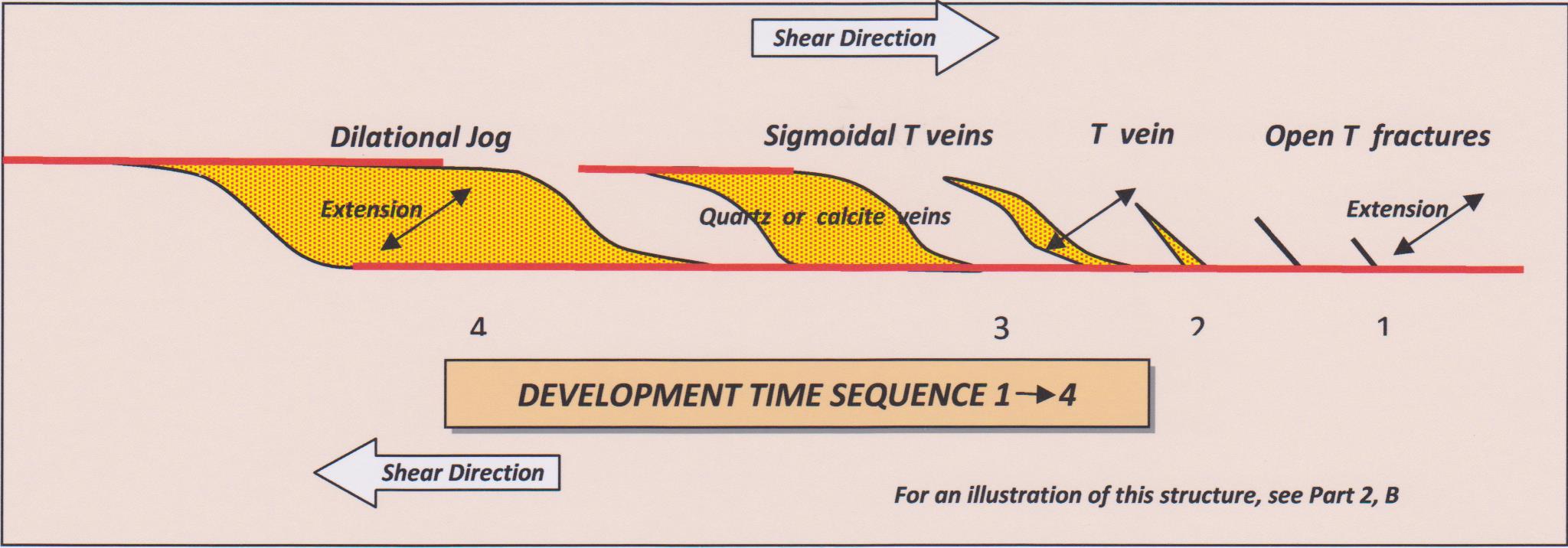
Figure 6:  Development of a dilational jog.

Dilational jogs can become very elongate. In these cases, it is likely that only the vein would be exposed and the nature of the structure as an offset in a shear zone would be hard, if not impossible, to spot in field exposure.

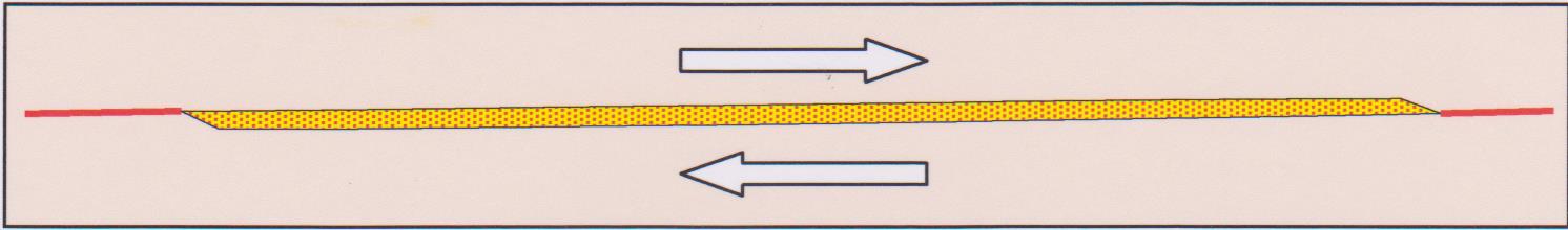
Figure 7:  An elongate dilational jog. In typical field exposure, only the vein would be exposed.

Veins occupying adjacent dilational jogs on the same shear surface can grow so as to overlap each other forming a stacked composite sheeted vein. The veins coat the surface like tiles or shingles on a roof – hence the common description of this structure as “shingling”.  A section through such stacked veins is shown below (figure 8). However, the most common field exposure is the face on view of the shear surface (figure 9).  Minerals comprising the veins (usually quartz or calcite) grow in the direction of extension, at right angles to the T surfaces.  This typically produces a strong mineral lineation in the direction of shear.

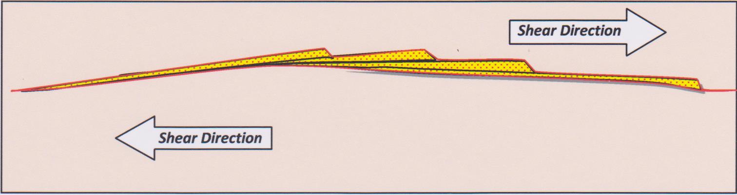
Figure 8:  Section through stacked dilational jogs. Note the overlapping veins look like tiles or shingles.  The steps are T surfaces.  They face the same way and indicate movement direction. The typical exposure of this structure is looking face on at the shear surface (figure 9).

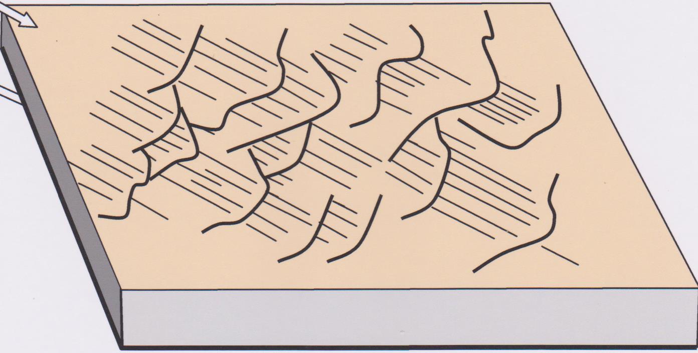
Figure 9:  Sketch of an exposed fault surface coated with thin sheets of overlapping tension veins. The leading edges of the veins  (T surfaces) form a series of asymmetric steps which face towards the direction of movement of the missing fault block. Within the veins, minerals have grown in the direction of extension (i.e. at right angles to the T surfaces) typically defining a strong lineation in the direction of shear. These are known as “fibres”.  For a photograph of this structure see Part 2 (E)

 

  Rotational or Non Co-Axial Strain

Within a zone of simple shear, stress axes are always oriented at 45° to the boundaries of the zone. Under  appropriate conditions the stress may produce any of the various structures shown in figure 5, above.  Structures start small then evolve and grow within the active shear zone over time. Any physical structure, once formed, will tend to be rotated by flow of material in the shear zone – even as it continues to grow. As a result, a long-lived planar structures will develop a distinctive sigmoidal shape, as  illustrated on the left of the diagram below.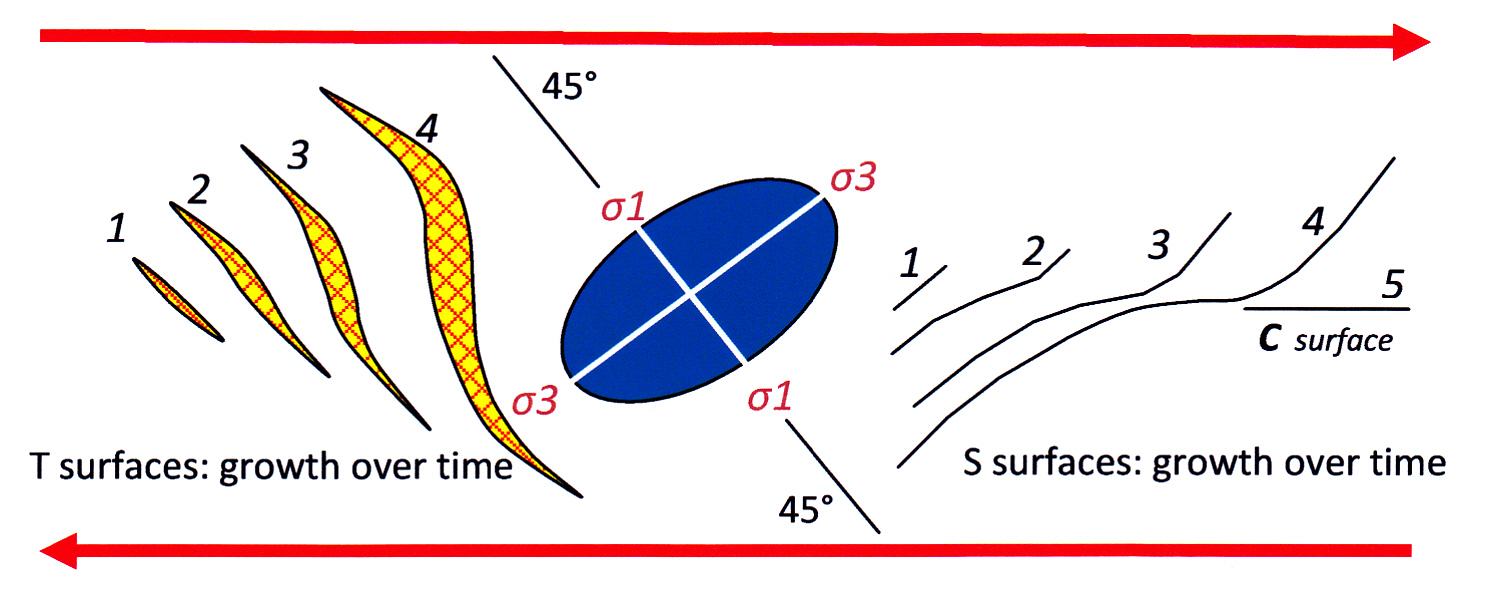    

Figure 10:  Progressive development of structures in a simple shear zone. The strain ellipsoid that exists at any instant is shown in blue . At left, are time stages (numbered 1-4) in the development of a quartz filled vein during continued dextral shear. At right, the progressive growth of an S surface (a ductile foliation) is exactly analogous to that of the vein although its orientation differs from the vein by 90°.

A tensional fracture initiates parallel to the stress axis σ1. That means it forms at 45° to the zone margin in a direction that is opposed to movement (stage 1, above left). The fracture begins where strain is greatest and that usually is in the centre of the zone. Fault fluids may deposit minerals (typically quartz or calcite) in the dilational fracture to form a vein. As shear movement continues, the early vein is physically rotated in a clockwise direction (stage 2).  Obviously, a vein in solid rock can only rotate if the material surrounding it is able to deform in a ductile manner.  Rotated tension veins are thus characteristic of deep level structures where a combination of brittle and ductile styles of deformation can operate, or where the fault fill material is relatively incompetent. This style of vein development contrasts with that of dilational jogs (see above), where brittle deformation predominates throughout vein development.

As it rotates, the vein continues to thicken and extend by growth at its tips. The new growth at the tips is controlled by the stress so is at 45° to the zone margins, making an angle to the older, now rotated, central part of the vein. The process continues (stages 3 & 4) with new growth at the extending tips always  forming at 45° to  the zone boundaries. The end result is the sigmoidal vein shape seen in stage 4.  Vein formation ceases when the bulk of the vein has rotated so much that there is no longer any resolved component of extension across it and is no longer able to accept new mineral deposition.

A compressive or S surface (the black lines of figure 10) such as a ductile foliation would seldom if ever form in a shear zone in the same place or at the same time as a tension fracture. However under appropriate conditions it will be initiated where strain is greatest – usually the central part. The surface forms parallel to the stress axis σ3, that is: at 45° to the zone boundaries in a direction congruent with shear movement (stage 1, above right). Its development over time now follows the same path as that of the tension vein with the early formed foliation being physically rotated towards parallelism with the boundaries of the shear zone whilst, at the same time, becoming extended by new growth at 45° to the zone boundaries. Once parallel with the principal shear direction it is known as a C surface. Shear movement takes place along C and low-angle S surfaces creating mineral lineation oriented in the direction of shear, as shown in the block diagram below.

 

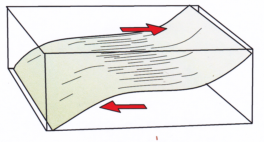
Figure 11: In ductile shear zones,  compression results in a foliation that initially forms at 45° to shear margins (S surfaces)  but in the centre of the zone becomes rotated into planes of laminar shear parallel to zone margins (C surfaces).  C surfaces typically are strongly lineated by oriented growth of elongate minerals or mineral aggregates.

In zones of strong ductile simple shear C and S surfaces are often partitioned into alternate laminae at millimeter to centimeter scale. This distinctive structure is known as S-C structure and is illustrated below. Such structures can provide an unequivocal sense of movement for the zone. However, in many examples, this type of structure is open to the alternative explanation that it a spaced cleavage, reflecting a second generation of folding, affecting an earlier S surface. To distinguish between the two explanations you need to know whether the C surfaces are parallel to the zone margins – not always easy when confronted with a small outcrop in the middle of a wide ductile shear zone.

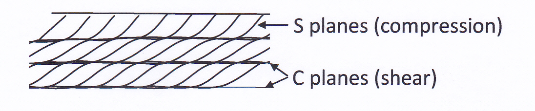Figure 12.  S-C structure in a ductile shear zone. This is interpreted as caused by dextral shear although the alternative explanation of a spaced cleavage is often also available. 

The above analysis is based on the assumption that structures in shear zones initiate in the central part of the zone where strain is greatest. However, in narrow shear zones with discrete and well defined margins the greatest strain may occur along the boundaries of the zone. A compressive S fabric in the centre of such zones will tend to rotate into parallelism with the shear direction (C surfaces) along the margins of the zone. This will yield shapes as shown below:

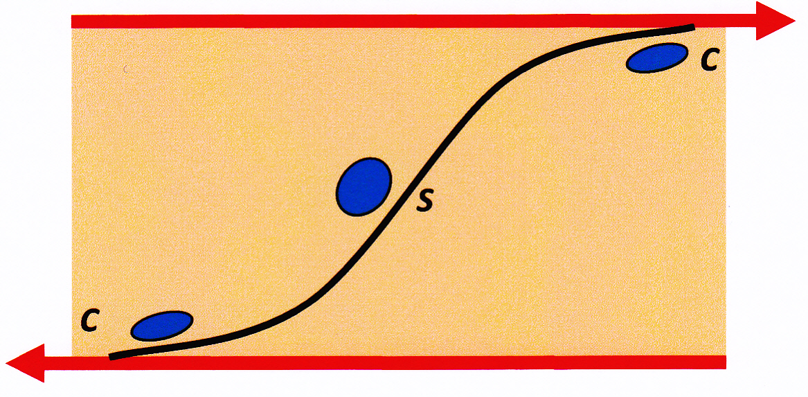
Figure 13: In shear zones with well defined margins simple shear strain is often greatest along the zone boundaries. In the centre of the zone compressive S foliation is at 45 degrees to the margins, but are rotated to parallelism with the shear direction (C surfaces) as they approach the contacts. Blue ellipses are the final strain ellipse showing the cumulative effects of both rotational and non-rotational strain. Where the shear zone is shallow-dipping and the movement produces a horizontal compression of the rocks, this structure is known as a thrust duplex (see illustrations G & H in Part 2).

Structures in high temperature ductile shear zones

In a ductile shear zone which has developed under conditions of high stress and temperature and across which a large amount of movement has taken place, almost all structure, no matter how initially formed, is rotated into parallelism with the shear surface C. However, minor inhomogeneity can lead to variations in strain that produce distinctive sense of movement structures. Some of these are illustrated below.

Figure 14: Structures in high temperature ductile shear zones. In A, a phenocryst or clast (blue dots) that has resisted deformation creates two low-pressure zones on its margins in which new mineral growth (coloured green) has occurred during deformation. Typically, the clasts range from a few millimeters to a few centimeters across. The asymmetry of these “tails” indicates the shear direction (compare this diagram with E). In B, the clast and attached tails has been physically rotated in the direction of shear, dragging the “tails” with it to create a spiral structure. In C, a marker surface in the shear zone (often an early formed quartz vein) is folded into an asymmetric fold pair. The axial planes of the folds mark S surfaces and their orientation relative to zone boundaries provides the sense of shear. In D, the clast has been split apart in a brittle fashion and new mineral growth (usually quartz or calcite) has grown in the low-pressure site between the separated pieces. This process is called boudinage (another French word).  In this case, the overall strain is one of  pure flattening and no sense of shear can be determined. Lastly, E shows symmetric “tails” of new mineral growth attached to the clast (compare to A). There is no sense of simple shear. Only a pure flattening strain in a direction normal to the boundaries of the ductile shear zone can be deduced.

Scaling it Up

It is important to remember that the widths of fault zones may range from a few millimeters to tens of kilometers. The structures shown on figure 6 therefore range in size from things that you might hope to see in a thin section or hand specimen to structures that might be shown on a regional geology map. Many structural geologists have used a diagram such as figure 6 as a template to lay on a regional map and so, from their strike orientation, read off the identity of the various structures. Such exercises are seldom convincing since knowledge of the strike of a structure provides insufficient evidence to enable its true nature to be determined.

Reidel shears (second order structures) can themselves be significant faults zones. Within these zones, third order stresses operate to provide third order structures. And, of course, within third order structures we can expect to find fourth order structures. And so on: it is an example of scale-dependent self-similarity, a fractal relationship. However, if we proceed much beyond third order structures, we have boxed the compass with the orientations of potential structures that can result from the original, first order, far field, causative stress.  At this point, in the real world, the whole analysis process usually breaks down into unconvincing complexity. There are just too many assumptions and selectable options.  Interpretations, although plausible, usually reflect wishful thinking. Analyses of this kind are however still attempted. They are generally known as Moody-Hill analyses after a pioneering and well known paper by these authors (on the San Andreas Fault Zone) published in 1956 (ref below).

Figure 15:  The relationships of First and Second Order Stress and Strain. This type of analysis, when applied at regional scale, is called a Moody-Hill analysis. Such analyses often invoke third, fourth and even higher orders of stress.

---